Age varying force of infection profiles • seropackage

library(seropackage)
knitr::opts_chunk$set(echo = TRUE)

We now consider the situation where FOI varies by age but the profile of infection remains constant over time, assuming no seroreversion in this article. Note that if we know the age of individuals, when they were born does not influence the trajectories of their seropositivities.


foiA <- c(0,3.65E-11,1.15E-07,5.21E-06,5.25134E-05,0.000250881,0.000776608,0.001819953,0.003524353,0.005950284,0.009069536,0.012780827,0.016934881,0.02136005,0.025883591,0.030346826,0.03461434,0.038578259,0.042158915,0.045303126,0.047981089,0.050182635,0.051913356,0.053190933,0.054041842,0.054498527,0.054597058,0.054375249,0.053871196,0.053122177,0.052163854,0.051029736,0.04975083,0.04835546,0.046869204,0.045314915,0.043712816,0.042080634,0.040433759,0.038785429,0.037146916,0.035527711,0.033935708,0.032377379,0.030857936,0.029381489,0.027951179,0.026569311,0.025237468,0.023956616,0.022727194,0.021549201,0.020422262,0.019345701,0.018318588,0.017339792,0.016408026,0.015521877,0.014679843,0.013880357,0.013121809,0.012402567,0.011720995,0.01107546,0.010464349,0.009886078,0.009339092,0.008821881,0.008332977,0.007870959,0.007434457,0.007022154,0.006632783,0.00626513,0.005918036,0.005590392,0.00528114,0.004989274,0.004713837,0.004453918,0.004208652,0.003977221,0.003758847,0.003552794,0.003358366,0.003174903)


year_survey <- 2024
age_cohorts <- c(16, 36, 44, 54, 64, 85)
birth_cohorts <- year_survey - age_cohorts

We assume that the force of infection is highest in those aged in their early 20s and that the age-profile of infection risk remains constant over time. For the age-varying FOI, the probability of being infected in a given year: $(1 - exp(-\bar \lambda_A))$

prob_infected_yr_df <- data.frame()

for(age in age_cohorts){
  for(a in 1:age){
    year <- (year_survey-age+a)
    prob_infected_yr <- 1-exp(-foiA[a]) # (1 - exp(-\bar \lambda_A))
    prob_infected_yr_df <- rbind(prob_infected_yr_df, c(age, prob_infected_yr, year))
  }
}

colnames(prob_infected_yr_df) <- c("age", "prob_infected", "year")
prob_infected_yr_df %>% 
  ggplot(aes(x = year, y = prob_infected, group = age, color = as.factor(age))) +
  geom_line() +
  scale_x_continuous(breaks = seq((year_survey-max(age_cohorts)), year_survey, by = 10)) +
  labs(x = "Year", y = "Pr(infected)") +
  guides(color = "none") +
  theme_bw() +
  theme(panel.grid = element_blank()) +
  coord_cartesian(expand = FALSE)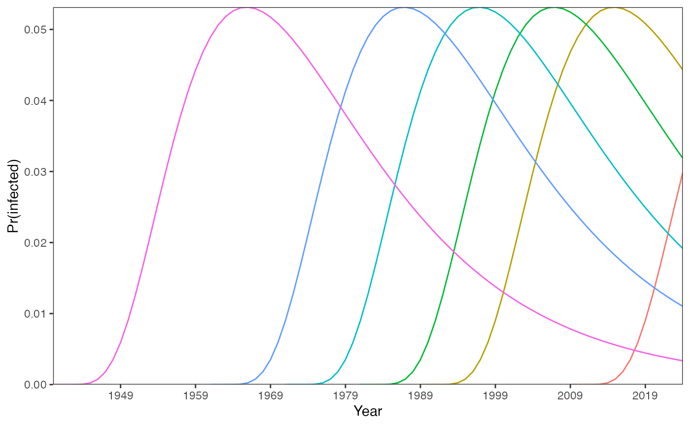

We track the progression of seropositivity over time for individuals from different birth cohorts up to the survey year (2024). The trajectories of seropositivity follow the same profile, regardless of when a cohort was born.


ages <- seq(1, length(foiA), 1)
year_survey <- 2024
age_cohorts <- c(16, 36, 44, 54, 64, 85)
birth_cohorts <- year_survey - age_cohorts

# (B) track seropositivity over time from birth:
# - calculate seropositivity for each year from birth to 2024:
prop_seropos_age_yr <- data.frame()

for(age in age_cohorts){
  # solution - eqn 35 in manuscript - sum of lambdas
  for(a in 1:age){
    year <- (year_survey-age) + a
    prop_seropos_age <- 1 - exp(-sum(foiA[1:a]))
    prop_seropos_age_yr <- rbind(prop_seropos_age_yr, c(age, prop_seropos_age, year))
  }
}

colnames(prop_seropos_age_yr) <- c("age", "prop_seropos", "year")
data_ends <- prop_seropos_age_yr %>% filter(year == 2024)

# - draw a line to show progression of exposure and infection:
ggplot() +
  geom_line(data = prop_seropos_age_yr, aes(x = year, y = prop_seropos, color = as.factor(age))) +
  geom_point(data = data_ends, aes(x = year, y = prop_seropos, shape = as.factor(age), 
                                   fill = as.factor(age)), size = 3) +
  scale_shape_manual(values = c(21,22,23,24,25,1)) +
  scale_y_continuous(labels = scales::percent_format(accuracy = 1), limits = c(0, 1),
                     breaks = seq(0, 1, by=0.1)) +
  scale_x_continuous(limits = c((year_survey-max(ages)), year_survey+1), 
                     breaks = seq((year_survey-max(ages)+1), (year_survey+1), 10)) +
  guides(fill = "none", color = "none", shape = "none") +
  coord_cartesian(expand = FALSE) +
  labs(x = "Year", y = "Seropositivity") +
  theme_bw() +
  theme(panel.grid = element_blank())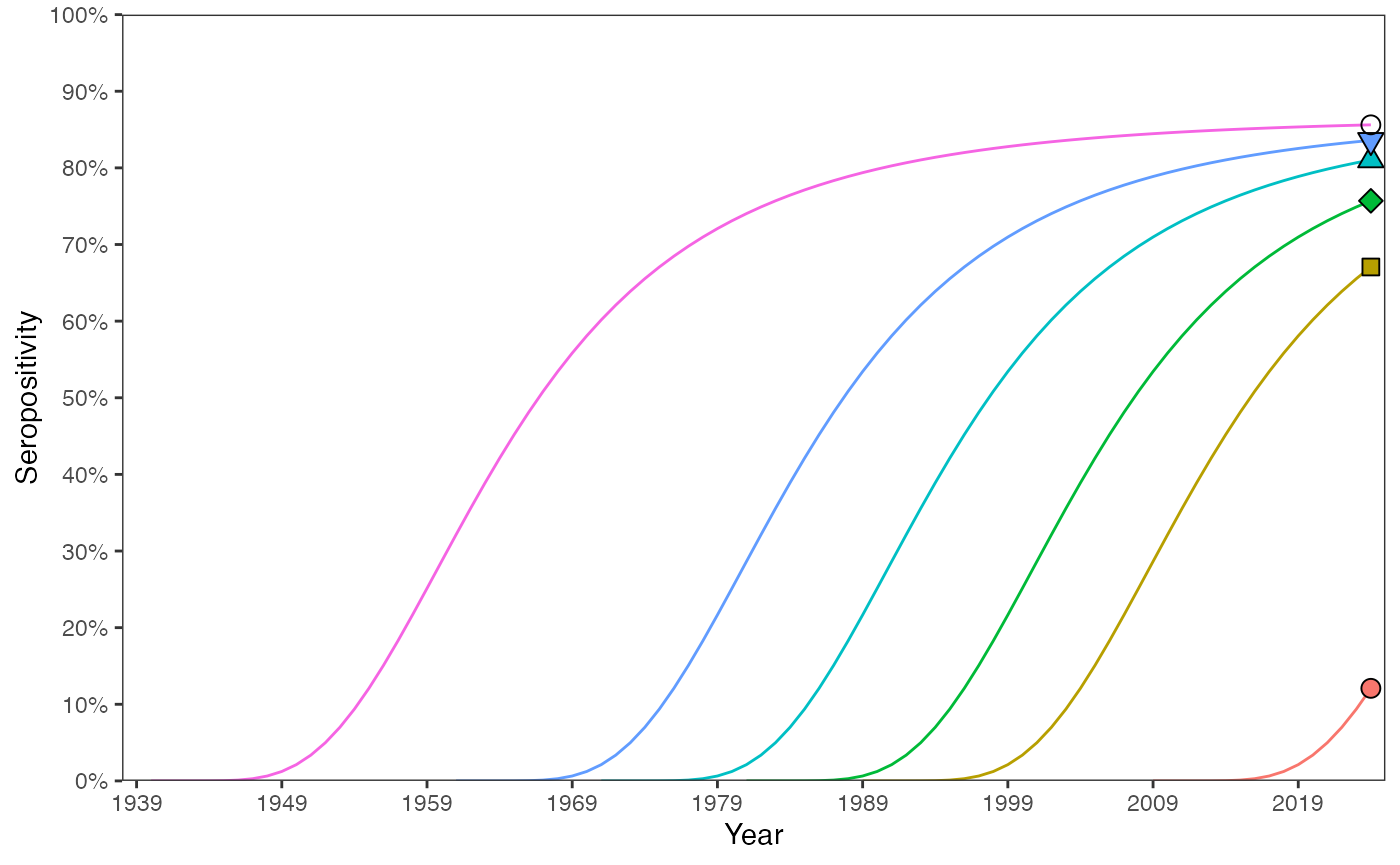

The dashed line shows the proportion seropositive for all age groups and the coloured markers correspond to the same 2024 values as shown in the above plot. We can see that older cohorts have higher seropositivity. This is generally true since when a new cohort is born, an existing cohort must have seropositivity of zero or higher. From then on, the two cohorts experience the same forces of infection.


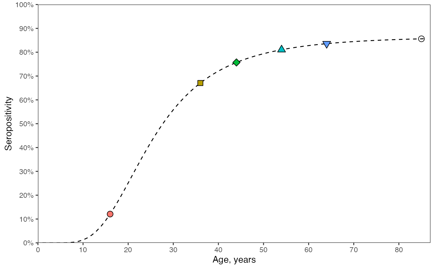
# (C) seropositivity in year of survey: T is constant. calculate the sum of lambdas upto the current age.

prop_seropos_age_yr2024 <- data.frame()

for(age in ages){
  # solution - eqn 26 in manuscript - sum of lambdas for T=2024
  prop_seropos_age <- 1 - exp(-sum(foiA[1:age]))
  prop_seropos_age_yr2024 <- rbind(prop_seropos_age_yr2024, c(age, prop_seropos_age))
}

colnames(prop_seropos_age_yr2024) <- c("age", "seropos")
data_cohorts <- prop_seropos_age_yr2024 %>% filter(age %in% age_cohorts)

ggplot() +
  geom_line(data = prop_seropos_age_yr2024, aes(x = age, y = seropos), linetype = "dashed") +
  geom_point(data = data_cohorts, aes(x = age, y = seropos, shape = as.factor(age), 
                                      fill = as.factor(age)), size = 3) +
  scale_shape_manual(values = c(21,22,23,24,25,1)) +
  scale_y_continuous(labels = scales::percent_format(accuracy = 1), limits = c(0,1),
                     breaks = seq(0,1,by=0.1)) +
  scale_x_continuous(limits = c(0, max(ages)+1), breaks = seq(0, max(ages), by=10)) +
  coord_cartesian(expand = FALSE) +
  labs(x = "Age, years", y = "Seropositivity") +
  guides(shape = "none", fill = "none") +
  theme_bw() +
  theme(panel.grid = element_blank())