Time varying force of infection profiles

library(seropackage)
knitr::opts_chunk$set(echo = TRUE)

We first generate a time-varying FOI, where the FOI is piecewise constant within a defined year. $~$

Probability of being infected in a given year: $$(1 - exp(-\bar \lambda_T))$$$~$

foiT <- rep(c(0.0,0.07,0.03,0.005,0.01,0.02), c(15,20,20,10,10,10))

prob_infected_yr <- function(lambdas){
  year = seq(1940,(1940+length(lambdas)-1),1)
  prob = 1-exp(-lambdas)
  
  tibble(year=year, prob=prob) %>% 
    ggplot(aes(x = year, y = prob)) +
    geom_line() +
    scale_y_continuous(breaks = seq(from = 0, to = 0.1, by = 0.01)) +
    labs(x = "Year", y = "Pr(infected in year)") +
    theme_bw() +
    theme(panel.grid = element_blank())
}

# Plot of the annual infection probabilities over time
prob_infected_yr(foiT)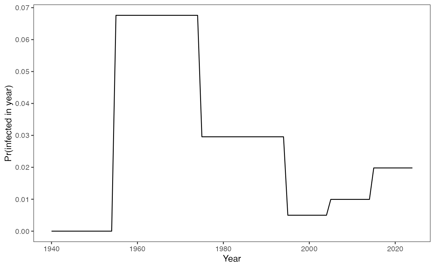

The solution of seropositivity trajectories for individuals from six birth cohorts across their lifespan up to 2024 are plotted. Seropositivity for each cohort is calculated iteratively by summing the FOI values year by year.

ages <- seq(1, length(foiT), 1)
sample_size <- 1000
m_exposure <- matrix(nrow = length(ages), ncol = length(ages))

for(i in seq_along(ages)) {
  n_zeros <- length(ages) - i
  n_ones <- i
  m_exposure[i, ] <- c(rep(0, n_zeros), rep(1, n_ones))
}

n_fois_exposed_per_obs <- rowSums(m_exposure)
foi_index_start_per_obs <- c(1, 1 + cumsum(n_fois_exposed_per_obs))
foi_index_start_per_obs <- foi_index_start_per_obs[-length(foi_index_start_per_obs)]
foi_indices <- unlist(map(seq(1, nrow(m_exposure), 1), ~which(m_exposure[., ]==1)))
fois_long <- foiT[foi_indices]

year_survey <- 2024
age_cohorts <- c(16, 36, 44, 54, 64, 85)
birth_cohorts <- year_survey - age_cohorts

# (B) track seropositivity over time from birth:
# - calculate seropositivity for each year from birth to 2024:
prop_seropos_age_yr <- data.frame()

for(age in age_cohorts){
  foi_start <- foi_index_start_per_obs[age]
  len <- n_fois_exposed_per_obs[age]
  foi_end <- foi_start + len - 1
  fois <- fois_long[foi_start:foi_end]
  # solution - eqn 20 in manuscript - sum of lambdas
  for(a in 1:age){
    year <- (year_survey-age) + a
    prop_seropos_age <- 1 - exp(-sum(fois[1:a]))
    prop_seropos_age_yr <- rbind(prop_seropos_age_yr, c(age, prop_seropos_age, year))
  }
}

colnames(prop_seropos_age_yr) <- c("age", "prop_seropos", "year")
data_ends <- prop_seropos_age_yr %>% filter(year == 2024)

# - draw a line to show progression of exposure and infection:
ggplot() +
  geom_line(data = prop_seropos_age_yr, aes(x = year, y = prop_seropos, color = as.factor(age))) +
  geom_point(data = data_ends, aes(x = year, y = prop_seropos, shape = as.factor(age), 
                                   fill = as.factor(age)), size = 3) +
  scale_shape_manual(values = c(21,22,23,24,25,1)) +
  scale_y_continuous(labels = scales::percent_format(accuracy = 1), limits = c(0, 1),
                     breaks = seq(0, 1, by=0.1)) +
  scale_x_continuous(limits = c((year_survey-max(ages)), year_survey+1), 
                     breaks = seq((year_survey-max(ages)+1), (year_survey+1), 10)) +
  guides(fill = "none", color = "none", shape = "none") +
  #coord_cartesian(expand = FALSE) +
  labs(x = "Year", y = "Seropositivity") +
  theme_bw() +
  theme(panel.grid = element_blank())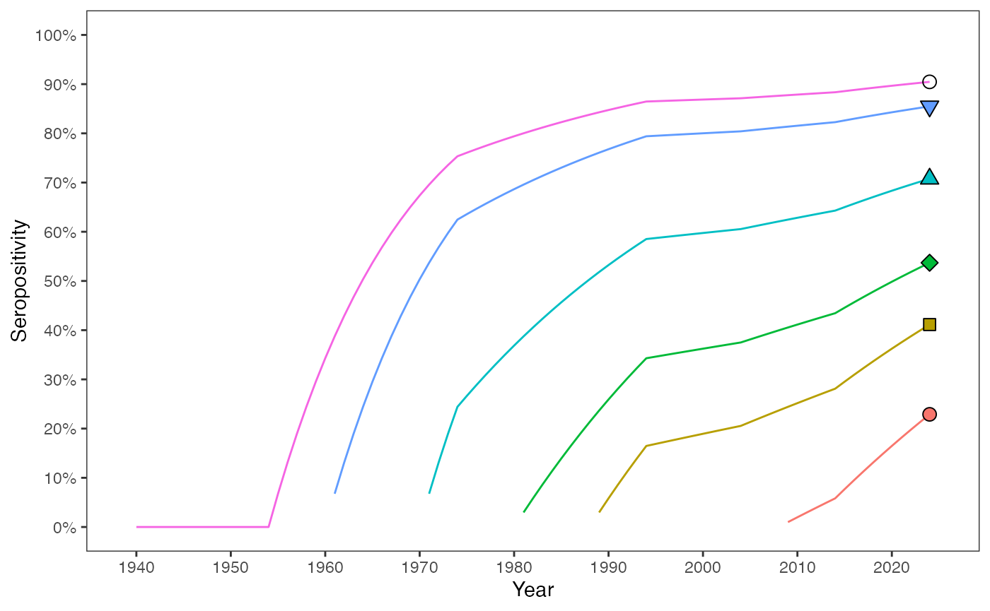

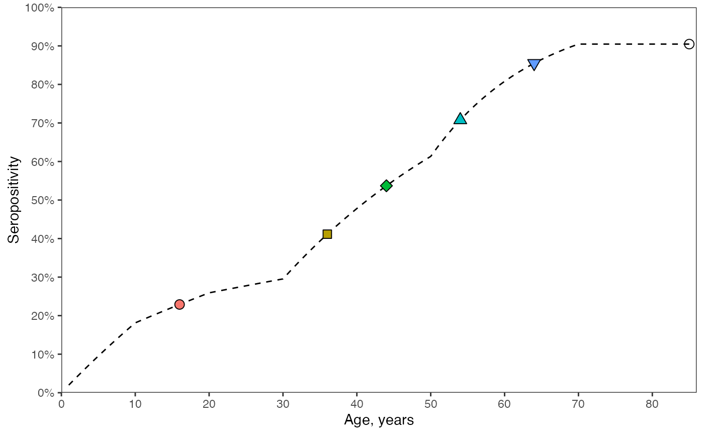
We now consider the seropositivity profile at a given time as a function of age. At a snapshot in time, we can determine a cross-sectional profile of seropositiity stratified by age. The coloured markers correspond to the serpositivities shown in 2024 in the previous plot.

# (C) seropositivity in year of survey: T is constant. calculate the sum of lambdas up to the current age.

prop_seropos_age_yr2024 <- data.frame()

for(age in ages){
  foi_start <- foi_index_start_per_obs[age]
  len <- n_fois_exposed_per_obs[age]
  foi_end <- foi_start + len - 1
  # solution - eqn 23 in manuscript - sum of lambdas for T=2024
  prop_seropos_age <- 1 - exp(-sum(fois_long[foi_start:foi_end]))
  prop_seropos_age_yr2024 <- rbind(prop_seropos_age_yr2024, c(age, prop_seropos_age))
}

colnames(prop_seropos_age_yr2024) <- c("age", "seropos")
data_cohorts <- prop_seropos_age_yr2024 %>% filter(age %in% age_cohorts)

# The serological age profile, in years, in the population in 2024.
ggplot() +
  geom_line(data = prop_seropos_age_yr2024, aes(x = age, y = seropos), linetype = "dashed") +
  geom_point(data = data_cohorts, aes(x = age, y = seropos, shape = as.factor(age), 
                                      fill = as.factor(age)), size = 3) +
  scale_shape_manual(values = c(21,22,23,24,25,1)) +
  scale_y_continuous(labels = scales::percent_format(accuracy = 1), limits = c(0,1),
                     breaks = seq(0,1,by=0.1)) +
  scale_x_continuous(limits = c(0, max(ages)+1), breaks = seq(0, max(ages), by=10)) +
  coord_cartesian(expand = FALSE) +
  labs(x = "Age, years", y = "Seropositivity") +
  guides(shape = "none", fill = "none") +
  theme_bw() +
  theme(panel.grid = element_blank())