Time varying force of infection with seroreversion profiles

library(seropackage)
knitr::opts_chunk$set(echo = TRUE)

For some infections, antibody levels wane with time below the limit of detection or seroreversion, defined in this context as a confirmed positive serologic test later testing negative [NF et al., 2022, Kayoko et al., 2021].

We follow the similar simulation method as in the model without seroreversion, a dashed horizontal line is added representing the seroreversion rate $\mu$. As before, the probability of being infected in a given year: $$(1 - exp(-\bar\lambda_T))$$.

foiT <- rep(c(0.0,0.07,0.03,0.005,0.01,0.02), c(15,20,20,10,10,10))

prob_infected_yr <- function(lambdas){
  year = seq(1940,(1940+length(lambdas)-1),1)
  prob = 1-exp(-lambdas)
  
  tibble(year=year, prob=prob) %>% 
    ggplot(aes(x = year, y = prob)) +
    geom_line() +
    geom_hline(yintercept = 0.015, linetype = 'dashed') +
    scale_y_continuous(breaks = seq(from = 0, to = 0.1, by = 0.01)) +
    labs(x = "Year", y = "Pr(infected in year)") +
    theme_bw() +
    theme(panel.grid = element_blank())
}

prob_infected_yr(foiT)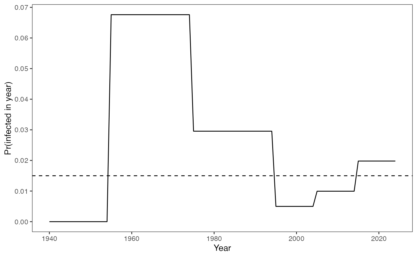

The seropositivity profiles are modified by including seroreversion into the model. Unlike the model without seroreversion, seropositivity of birth-cohorts decreases over a time interval, when the proportion of seropositive individuals becoming seronegative exceeds the proportion of seronegative individuals becoming infected (Eq.31 in the manuscript).

ages <- seq(1, length(foiT), 1)
sample_size <- 100
m_exposure <- matrix(nrow = length(ages), ncol = length(ages))

for(i in seq_along(ages)) {
  n_zeros <- length(ages) - i
  n_ones <- i
  m_exposure[i, ] <- c(rep(0, n_zeros), rep(1, n_ones))
}

n_fois_exposed_per_obs <- rowSums(m_exposure)
foi_index_start_per_obs <- c(1, 1 + cumsum(n_fois_exposed_per_obs))
foi_index_start_per_obs <- foi_index_start_per_obs[-length(foi_index_start_per_obs)]
foi_indices <- unlist(map(seq(1, nrow(m_exposure), 1), ~which(m_exposure[., ]==1)))
fois_long <- foiT[foi_indices]

year_survey <- 2024
age_cohorts <- c(16, 36, 44, 54, 64, 85)
birth_cohorts <- year_survey - age_cohorts

# (B) track seropositivity over time from birth:
# - calculate seropositivity for each year from birth to 2024:
prop_seropos_age_yr <- data.frame()
mu <- 0.015

for(age in age_cohorts){
  foi_start <- foi_index_start_per_obs[age]
  len <- n_fois_exposed_per_obs[age]
  foi_end <- foi_start + len - 1
  fois <- fois_long[foi_start:foi_end]
  prop_seropos_age <- 0
  for(a in 1:age){
    year <- (year_survey-age) + a
    # solves ODE exactly within pieces
    lambda <- fois[a]
    prop_seropos_age <- (1 / (lambda + mu)) * exp(-(lambda + mu)) * (lambda * (exp(lambda + mu) - 1) + prop_seropos_age * (lambda + mu))
    
    prop_seropos_age_yr <- rbind(prop_seropos_age_yr, c(age, prop_seropos_age, year))
  }
  

}

colnames(prop_seropos_age_yr) <- c("age", "prop_seropos", "year")
data_ends <- prop_seropos_age_yr %>% filter(year == 2024)

# - draw a line to show progression of exposure and infection:
ggplot() +
  geom_line(data = prop_seropos_age_yr, aes(x = year, y = prop_seropos, color = as.factor(age))) +
  geom_point(data = data_ends, aes(x = year, y = prop_seropos, shape = as.factor(age), 
                                   fill = as.factor(age)), size = 3) +
  scale_shape_manual(values = c(21,22,23,24,25,1)) +
  scale_y_continuous(labels = scales::percent_format(accuracy = 1), limits = c(0, 1),
                     breaks = seq(0, 1, by=0.1)) +
  scale_x_continuous(limits = c((year_survey-max(ages)), year_survey+1), 
                     breaks = seq((year_survey-max(ages)+1), (year_survey+1), 10)) +
  guides(fill = "none", color = "none", shape = "none") +
  #coord_cartesian(expand = FALSE) +
  labs(x = "Year", y = "Seropositivity") +
  theme_bw() +
  theme(panel.grid = element_blank())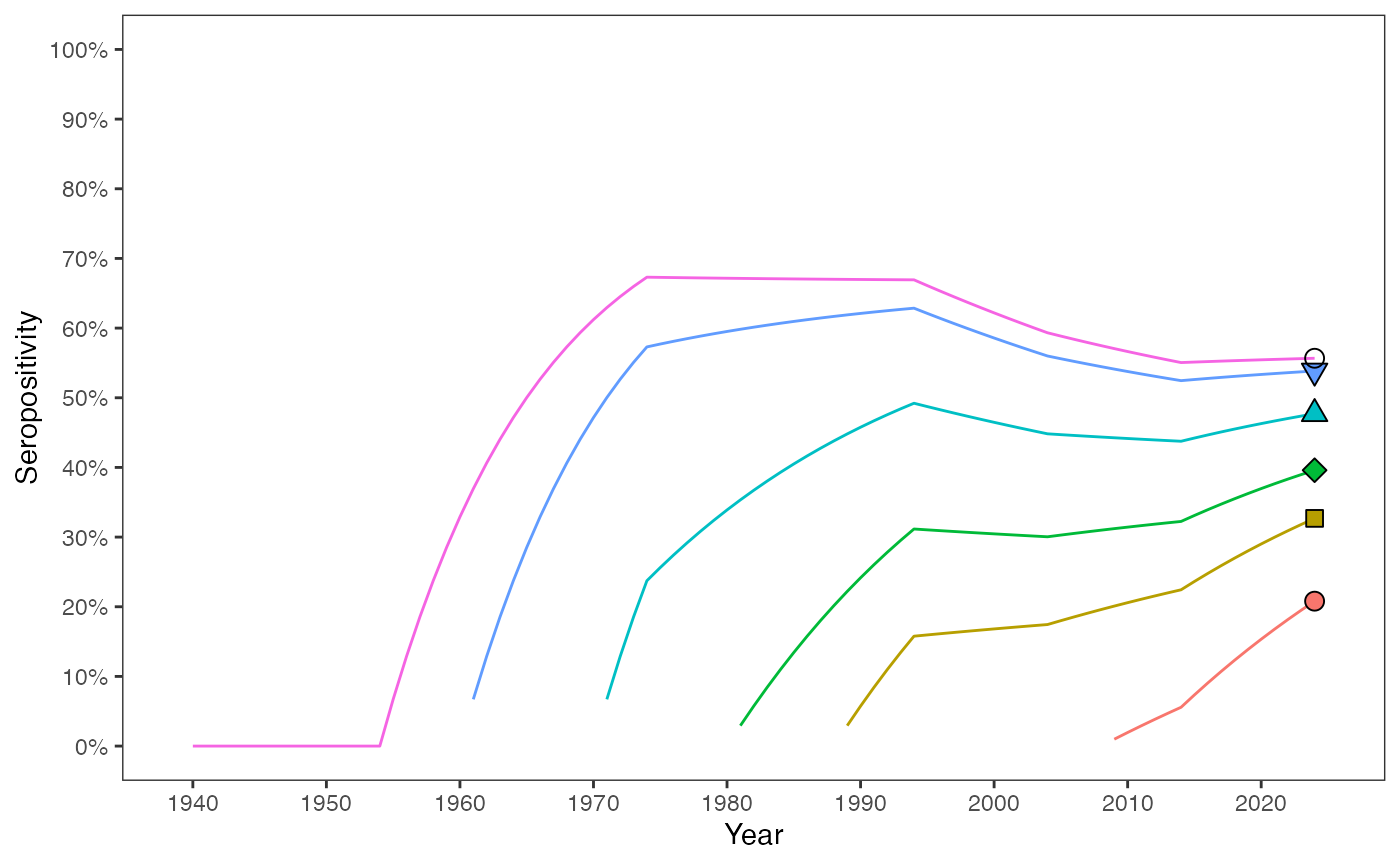

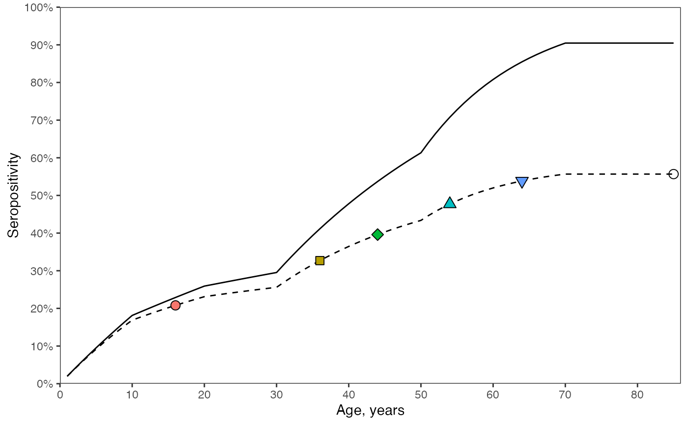
Similarly, if we take a snapshot at a time, the inclusion of seroreversion in the model leads to lower seropositivity at each age. The solid line shows the model solution if the rate of seroreversion were zero.

# (C) seropositivity in year of survey: T is constant. calculate the sum of lambdas upto the current age.

# 1) with seroreversion:
prop_seropos_age_yr2024 <- data.frame()
mu <- 0.015

for(age in ages){
  foi_start <- foi_index_start_per_obs[age]
  len <- n_fois_exposed_per_obs[age]
  foi_end <- foi_start + len - 1
  fois <- fois_long[foi_start:foi_end]
  # solution - for T=2024
  
  prop_seropos_age <- 0
  for(a in 1:age){
    # solves ODE exactly within pieces
    lambda <- fois[a]
    prop_seropos_age <- (1 / (lambda + mu)) * exp(-(lambda + mu)) * (lambda * (exp(lambda + mu) - 1) + prop_seropos_age * (lambda + mu))
    
  }
  prop_seropos_age_yr2024 <- rbind(prop_seropos_age_yr2024, c(age, prop_seropos_age))
  
}

colnames(prop_seropos_age_yr2024) <- c("age", "seropos")
data_cohorts <- prop_seropos_age_yr2024 %>% filter(age %in% age_cohorts)


# 2) without seroreversion
prop_seropos_age_yr2024_noSerorev <- data.frame()
mu <- 0.0

for(age in ages){
  foi_start <- foi_index_start_per_obs[age]
  len <- n_fois_exposed_per_obs[age]
  foi_end <- foi_start + len - 1
  fois <- fois_long[foi_start:foi_end]
  # solution - for T=2024
  
  prop_seropos_age <- 0
  for(a in 1:age){
    # solves ODE exactly within pieces
    lambda <- fois[a]
    prop_seropos_age <- (1 / (lambda + mu)) * exp(-(lambda + mu)) * (lambda * (exp(lambda + mu) - 1) + prop_seropos_age * (lambda + mu))
    
  }
  prop_seropos_age_yr2024_noSerorev <- rbind(prop_seropos_age_yr2024_noSerorev, c(age, prop_seropos_age))
  
}

colnames(prop_seropos_age_yr2024_noSerorev) <- c("age", "seropos")
prop_seropos_age_yr2024_noSerorev$seropos[is.na(prop_seropos_age_yr2024_noSerorev$seropos)] <- tail(prop_seropos_age_yr2024_noSerorev$seropos[!is.na(prop_seropos_age_yr2024_noSerorev$seropos)], 1)


# plot both models with and without seroreversion

ggplot() +
  geom_line(data = prop_seropos_age_yr2024, aes(x = age, y = seropos), linetype = "dashed") +
  geom_point(data = data_cohorts, aes(x = age, y = seropos, shape = as.factor(age), 
                                      fill = as.factor(age)), size = 3) +
  geom_line(data = prop_seropos_age_yr2024_noSerorev, aes(x = age, y = seropos)) +
  scale_shape_manual(values = c(21,22,23,24,25,1)) +
  scale_y_continuous(labels = scales::percent_format(accuracy = 1), limits = c(0,1),
                     breaks = seq(0,1,by=0.1)) +
  scale_x_continuous(limits = c(0, max(ages)+1), breaks = seq(0, max(ages), by=10)) +
  coord_cartesian(expand = FALSE) +
  labs(x = "Age, years", y = "Seropositivity") +
  guides(shape = "none", fill = "none") +
  theme_bw() +
  theme(panel.grid = element_blank())