Time and age varying force of infection profiles

library(seropackage)
knitr::opts_chunk$set(echo = TRUE)

In this article, the FOI varies as a product of time- and age-specific patterns, meaning persistent age-related patterns that fluctuate temporally. We do not consider serorevernsion in this article, but it is included in the manuscript.

We assume that $u(.)$ and $v(.)$ are both piecewise-constant, where $u(.)$ is a function of age and $v(.)$ is a function of time. The peak of $u(.)$ is chosen to be in the early 20s. At the same time, we allow a rapid increase in the level of transmission, starting in the year 1980.

year_survey <- 2024
age_cohorts <- c(16, 32, 44, 52, 62, 72, 85)
birth_cohorts <- year_survey - age_cohorts

# piecewise constant rates: v(t) - for time;  
v <- c(rep(0.1, 42), rep(1, 43))

# piecewise constant rates: u(a) - for age:
mu <- 3.5; sigma <- 0.5 # parameters for LogNormal distribution
## Generate values using LogNormal distribution and compute PDF
x_values <- seq(1, 85, 1)
u <- 2 * dlnorm(x_values, meanlog = mu, sdlog = sigma)
plot(u, type="l") # age

plot(v, type="l") # time

The probability of being infected at a given year for an arbitrary birth cohort is defined as Eq.48 in the manuscript.

# calculate cumulative probability of being infected and proportion seropositive:
prop_infected_df <- data.frame()
prop_seropos_df <- data.frame()

for(age in age_cohorts){
  print(age)
  years = rev(head(year_survey:(year_survey-age), -1)) # years of exposure by the cohort
  cohort = (year_survey - age) # birth year
  v_vector = tail(v, age)
  for(t in years){
    print(t)
    sum_foi = 0
    for(i in 1:(t-cohort)){
      print(i)
      foi = (u[i] * v_vector[i])
      sum_foi = sum_foi + foi
    }
    prop_infected_df = rbind(prop_infected_df, c(age, cohort, t, foi))
    
    prop_seropos = 1-exp(-sum_foi)
    print(prop_seropos)
    prop_seropos_df = rbind(prop_seropos_df, c(age, cohort, t, prop_seropos))
  }
}

colnames(prop_infected_df) <- c("age", "birth_yr", "year", "sum_foi_pdt")
colnames(prop_seropos_df) <- c("age", "birth_yr", "year", "prop_seropos")

# calculate discrete age probability of being infected and proportion seropositive:
ages <- 1:85
prop_infected_df2 <- data.frame()
prop_seropos_df2 <- data.frame()

for(age in ages){
  print(age)
  years = rev(head(year_survey:(year_survey-age), -1)) # years of exposure by the cohort
  cohort = (year_survey - age) # birth year
  v_vector = tail(v, age)
  for(t in years){
    print(t)
    sum_foi = 0
    for(i in 1:(t-cohort)){
      print(i)
      foi = (u[i] * v_vector[i])
      sum_foi = sum_foi + foi
    }
    prop_infected_df2 = rbind(prop_infected_df2, c(age, cohort, t, foi))
    
    prop_seropos = 1-exp(-sum_foi)
    print(prop_seropos)
    prop_seropos_df2 = rbind(prop_seropos_df2, c(age, cohort, t, prop_seropos))
  }
}

colnames(prop_infected_df2) <- c("age", "birth_yr", "year", "sum_foi_pdt")
colnames(prop_seropos_df2) <- c("age", "birth_yr", "year", "prop_seropos")

Figures:

This figure shows the probability of becoming infected per year for seven birth-cohorts.

# Fig1A: probability of being infected in one's lifetime:

prop_infected_df %>% 
  ggplot(aes(x = year, y = sum_foi_pdt, group = as.factor(age), 
             color = as.factor(age))) +
  geom_line() +
  labs(x = "Year", y = "Pr(infected)", color = "Age") + 
  theme_bw() +
  theme(legend.position = "none")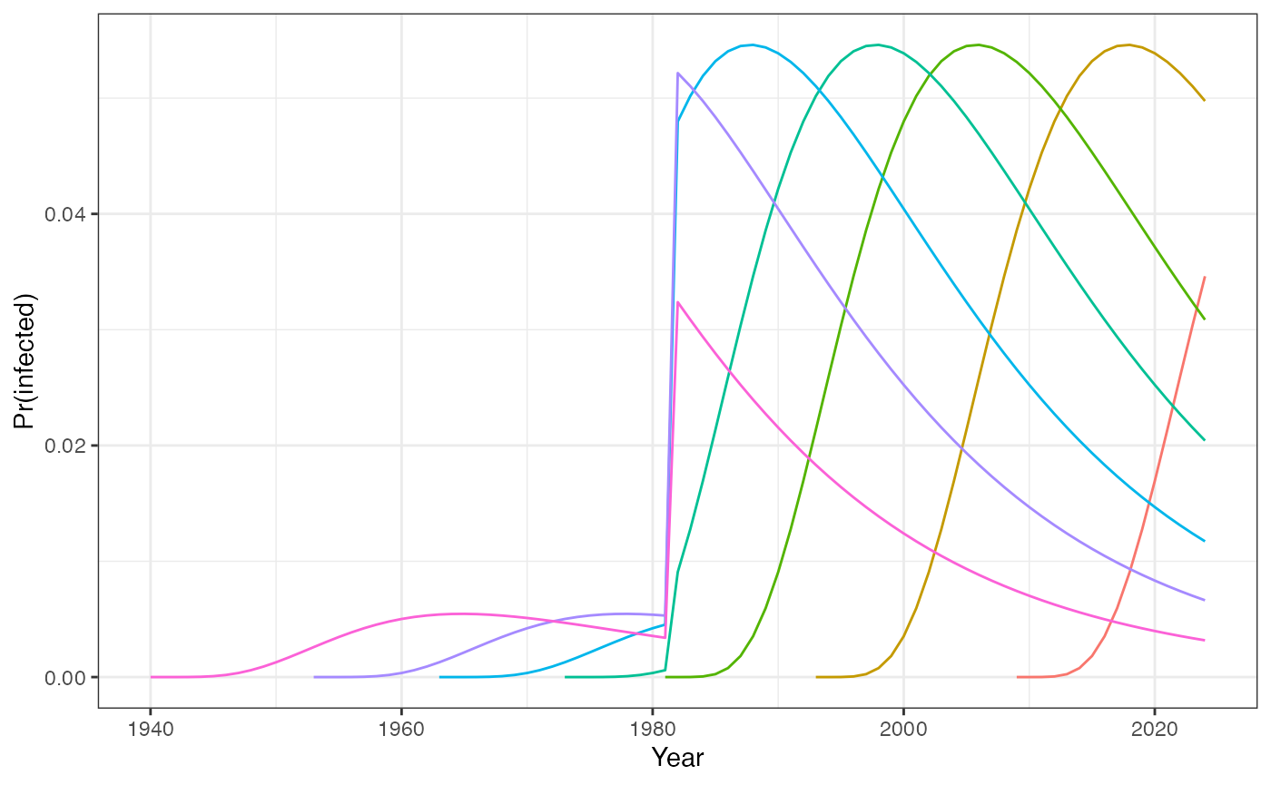

The upward shift in transmission in 1980 means that the individuals born during the period of elevated transmission experience a disproportionately higher risk of infection and seropositive proportion of these cohorts can exceed those of older individuals.

# Fig 1B: seropositivity in one's lifetime:

ggplot(prop_seropos_df, aes(x = year, y = prop_seropos, group = as.factor(age), 
             color = as.factor(age))) +
  geom_line() +
  geom_point(data = prop_seropos_df %>% dplyr::filter(year == 2024), 
             aes(x = year, y = prop_seropos, group = as.factor(age), 
                 fill = as.factor(age), shape = as.factor(age)), size = 3) +
  scale_shape_manual(values = c("16"=0,"32"=1,"44"=25,"52"=17,"62"=23,"72"=15,"85"=16)) +
  scale_y_continuous(labels = scales::percent) +
  labs(x = "Year", y = "Seropositivity") +
  theme_bw() +
  theme(legend.position = "none")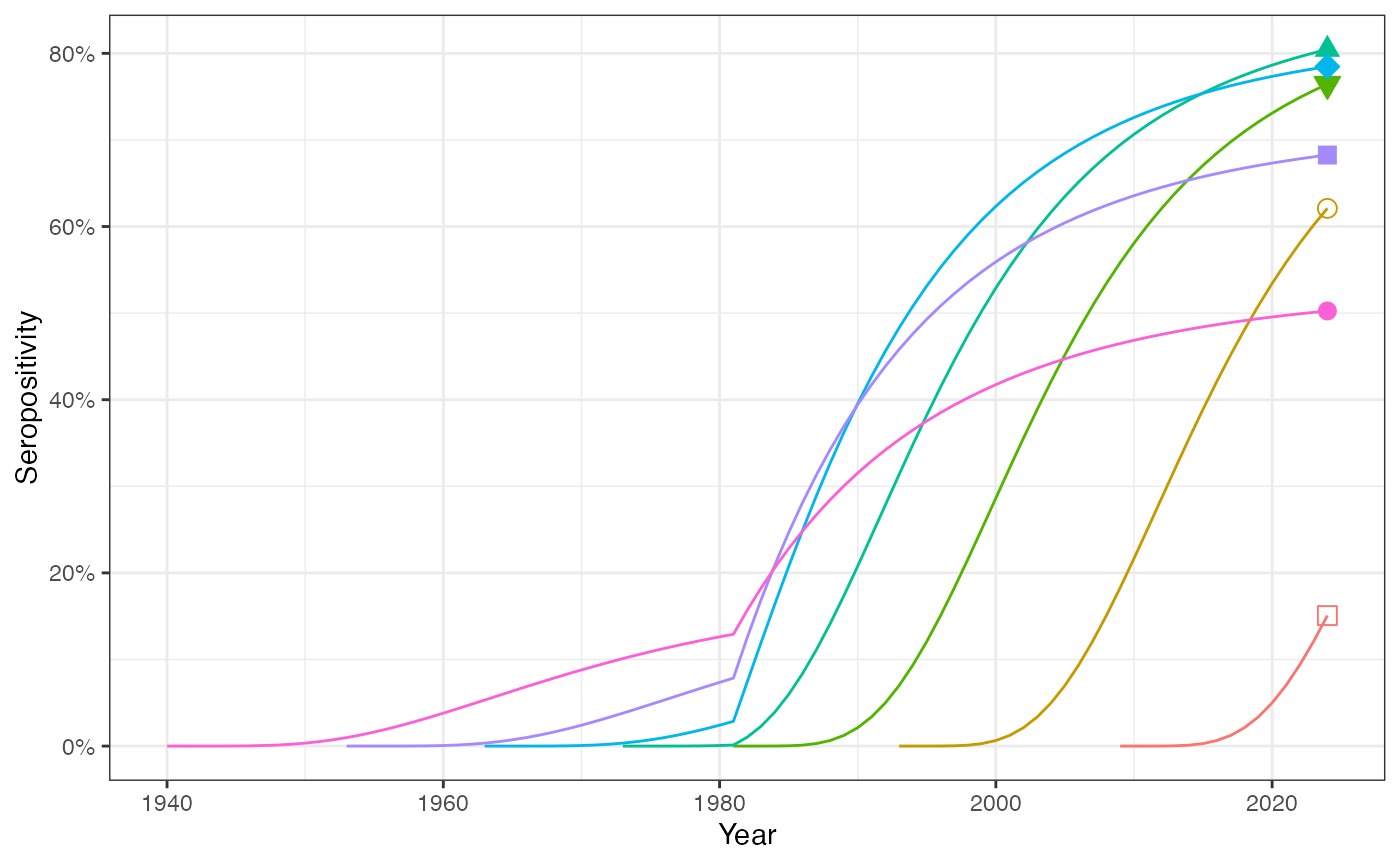

$~$

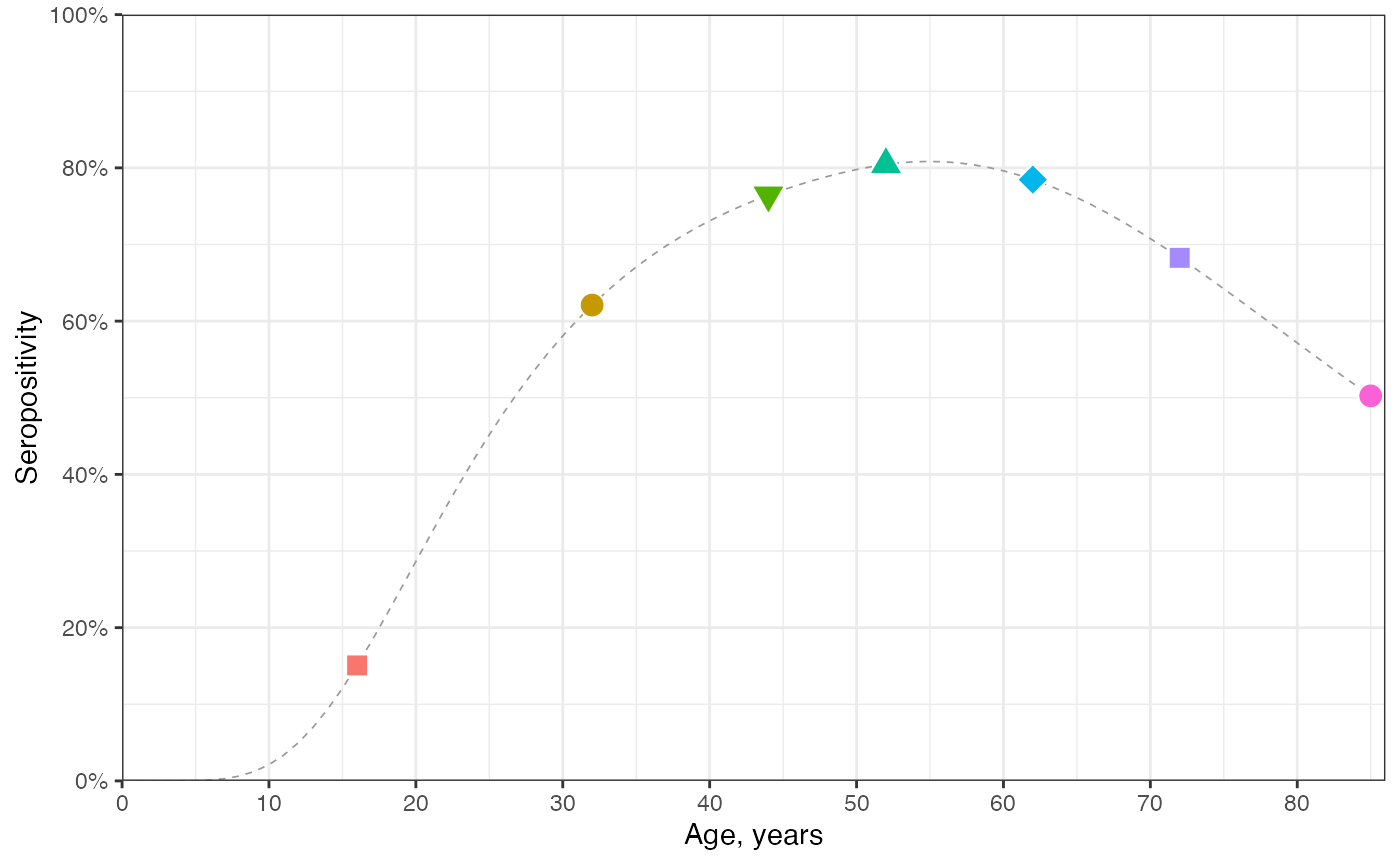
# Fig1C: seropositivity in year 2024:

prop_seropos_age_yr2024 <- prop_seropos_df2 %>% dplyr::filter(year == 2024)

ggplot() +
  geom_line(data = prop_seropos_age_yr2024, aes(x = age, y = prop_seropos), color = "grey60", 
            linewidth = 0.3, linetype = "dashed") +
  geom_point(data = dplyr::filter(prop_seropos_age_yr2024, age %in% c(age_cohorts)),
             aes(x = age, y = prop_seropos, shape = as.factor(age), fill = as.factor(age)),
             size = 4, color = "white") +
  scale_shape_manual(values = c("16"=22,"32"=21,"44"=25,"52"=24,"62"=23,"72"=22,"85"=21)) +
  scale_y_continuous(limits = c(0,1), breaks = seq(0,1,by=0.2), labels = scales::percent) +
  scale_x_continuous(limits = c(0, max(age_cohorts)+1), breaks = seq(0, max(age_cohorts), by=10)) +
  coord_cartesian(expand = FALSE) +
  labs(x = "Age, years", y = "Seropositivity") +
  theme_bw() +
  theme(legend.position = "none")